Python机器学习13 |
您所在的位置:网站首页 › Python里面的成分矩阵 › Python机器学习13 |
Python机器学习13
|
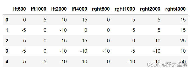
本系列所有的代码和数据都可以从陈强老师的个人主页上下载:Python数据程序 参考书目:陈强.机器学习及Python应用. 北京:高等教育出版社, 2021. 本系列基本不讲数学原理,只从代码角度去让读者们利用最简洁的Python代码实现机器学习方法。 无监督学习就是没有y,让算法从特征变量x里面自己寻找特征。 本节开始无监督学习的方法,经典统计学的主成分分析,可以将数据进行线性变化从而进行降维,用少数几个变量代替原始的很多的变量。但是主成分不能进行变量筛选,因为新的变量是原始变量的线性组合,失去了原有的含义。而和主成分很像的因子分析可以进行部分解释。 主成分分析的Python案例采用一个听力的数据集,导入包和数据: import numpy as np import pandas as pd import matplotlib.pyplot as plt import seaborn as sns from sklearn.preprocessing import StandardScaler from sklearn.decomposition import PCA from sklearn.model_selection import cross_val_score from sklearn.linear_model import LinearRegression from sklearn.model_selection import LeaveOneOut from mpl_toolkits import mplot3d audiometric = pd.read_csv('audiometric.csv') audiometric.shape audiometric.head()数据长这样
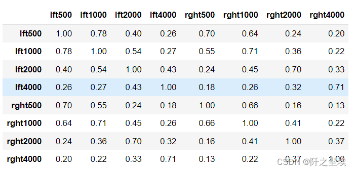
计算其相关系数 pd.options.display.max_columns = 10 round(audiometric.corr(), 2)
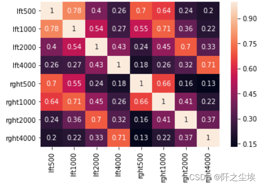
画出相关系数矩阵热力图 sns.heatmap(round(audiometric.corr(), 2),annot=True)
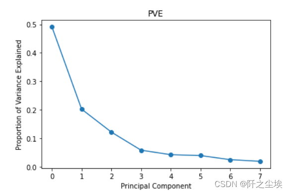
数据标准化 scaler = StandardScaler() scaler.fit(audiometric) X = scaler.transform(audiometric)主成分pca拟合 model = PCA() model.fit(X) #每个主成分能解释的方差 model.explained_variance_ #每个主成分能解释的方差的百分比 model.explained_variance_ratio_ #可视化 plt.plot(model.explained_variance_ratio_, 'o-') plt.xlabel('Principal Component') plt.ylabel('Proportion of Variance Explained') plt.title('PVE')
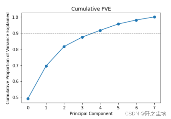
画累计百分比,这样可以判断选几个主成分 plt.plot(model.explained_variance_ratio_.cumsum(), 'o-') plt.xlabel('Principal Component') plt.ylabel('Cumulative Proportion of Variance Explained') plt.axhline(0.9, color='k', linestyle='--', linewidth=1) plt.title('Cumulative PVE')
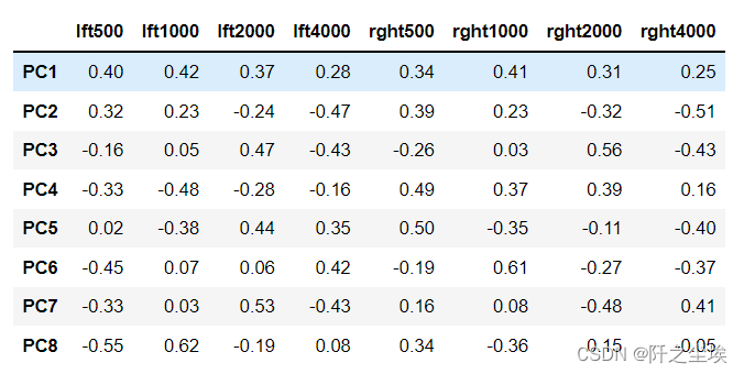
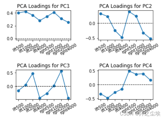
4个主成分能解释到90%以上了 主成分核载矩阵 #主成分核载矩阵 model.components_ columns = ['PC' + str(i) for i in range(1, 9)] pca_loadings = pd.DataFrame(model.components_, columns=audiometric.columns, index=columns) round(pca_loadings, 2) 该矩阵展示了每个主成分是原始数据的线性组合,以及线性的系数 画图展示 # Visualize pca loadings fig, ax = plt.subplots(2, 2) plt.subplots_adjust(hspace=1, wspace=0.5) for i in range(1, 5): ax = plt.subplot(2, 2, i) ax.plot(pca_loadings.T['PC' + str(i)], 'o-') ax.axhline(0, color='k', linestyle='--', linewidth=1) ax.set_xticks(range(8)) ax.set_xticklabels(audiometric.columns, rotation=30) ax.set_title('PCA Loadings for PC' + str(i))
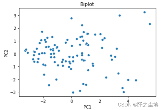
计算每个样本的主成分得分 # PCA Scores pca_scores = model.transform(X) pca_scores = pd.DataFrame(pca_scores, columns=columns) pca_scores.shape pca_scores.head() #前两个主成分的可视化 # visualize pca scores via biplot sns.scatterplot(x='PC1', y='PC2', data=pca_scores) plt.title('Biplot')
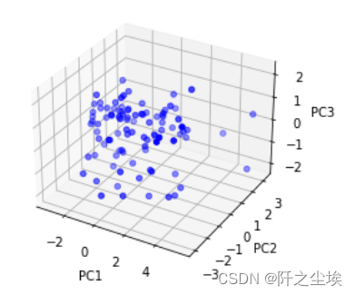
三个主成分的可视化,三维图 # Visualize pca scores via triplot fig = plt.figure() ax = fig.add_subplot(111, projection='3d') ax.scatter(pca_scores['PC1'], pca_scores['PC2'], pca_scores['PC3'], c='b') ax.set_xlabel('PC1') ax.set_ylabel('PC2') ax.set_zlabel('PC3')
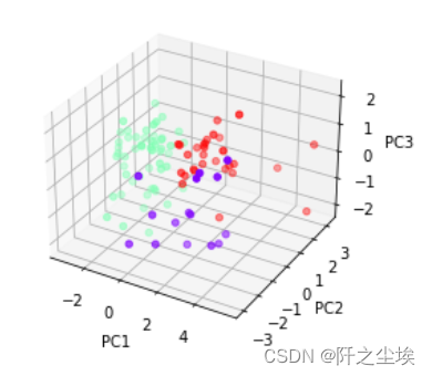
利用K均值聚类对三个主成分聚类,可视化 from sklearn.cluster import KMeans model = KMeans(n_clusters=3, random_state=1, n_init=20) model.fit(X) model.labels_ fig = plt.figure() ax = fig.add_subplot(111, projection='3d') ax.scatter(pca_scores['PC1'], pca_scores['PC2'], pca_scores['PC3'], c=model.labels_, cmap='rainbow') ax.set_xlabel('PC1') ax.set_ylabel('PC2') ax.set_zlabel('PC3')
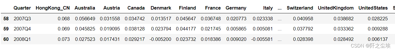
使用中国香港的季度增长率的数据集进行主成分回归,读取数据,考察形状 growth = pd.read_csv('growth.csv') growth.shape growth.head(3) growth.tail(3)
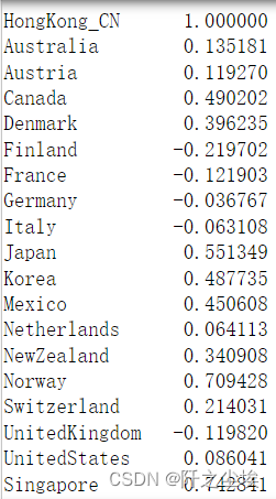
x为和中国香港相邻或有密切来往的24个国家的经济增长率。 #设置时间索引 growth.index = growth['Quarter'] growth = growth.drop(columns=['Quarter']) #计算香港和其他地区的相关系数 # Correlation between HK's growth rate and other countries growth.corr().iloc[:, 0]
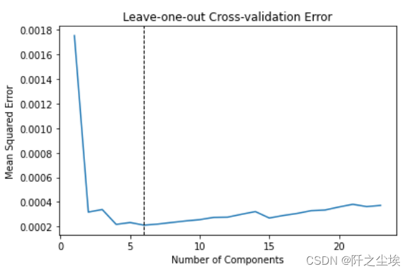
划分训练测试集,手工划分,前44个数据作为训练集,后面测试集。然后标准化 X_train = growth.iloc[:44, 1:] X_train.shape X_test = growth.iloc[44:, 1:] X_test.shape y_train = growth.iloc[:44, 0] y_test = growth.iloc[44:, 0] scaler = StandardScaler() scaler.fit(X_train) X_train = scaler.transform(X_train) X_test = scaler.transform(X_test)使用留一交叉验证选择误差最小的时候的主成分个数 scores_mse = [] for k in range(1, 24): model = PCA(n_components=k) model.fit(X_train) X_train_pca = model.transform(X_train) loo = LeaveOneOut() mse = -cross_val_score(LinearRegression(), X_train_pca, y_train, cv=loo, scoring='neg_mean_squared_error') scores_mse.append(np.mean(mse)) min(scores_mse) index = np.argmin(scores_mse) index plt.plot(range(1, 24), scores_mse) plt.axvline(index + 1, color='k', linestyle='--', linewidth=1) plt.xlabel('Number of Components') plt.ylabel('Mean Squared Error') plt.title('Leave-one-out Cross-validation Error') plt.tight_layout()
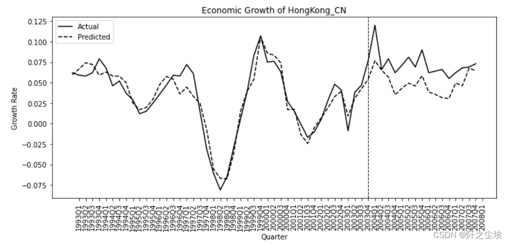
主成分个数为6时最小,下面使用六个主成分回归 model = PCA(n_components = index + 1) model.fit(X_train) #得到主成分得分 X_train_pca = model.transform(X_train) X_test_pca = model.transform(X_test) X_train_pca #进行线性回归拟合 reg = LinearRegression() reg.fit(X_train_pca, y_train) #全样本预测 X_pca = np.vstack((X_train_pca, X_test_pca)) X_pca.shape pred = reg.predict(X_pca) y = growth.iloc[:, 0] #可视化 plt.figure(figsize=(10, 5)) ax = plt.gca() plt.plot(y, label='Actual', color='k') plt.plot(pred, label='Predicted', color='k', linestyle='--') plt.xticks(range(1, 62)) ax.set_xticklabels(growth.index, rotation=90) plt.axvline(44, color='k', linestyle='--', linewidth=1) plt.xlabel('Quarter') plt.ylabel('Growth Rate') plt.title("Economic Growth of HongKong_CN") plt.legend(loc='upper left') plt.tight_layout()
在44之前没有政策,曲线拟合效果好,44之后开始 政策实施,真实值大于拟合值,说明政策有效,促进了中国香港经济的发展。 |
【本文地址】
今日新闻 |
推荐新闻 |